CREATION
OF GANTT CHART WITH THE USE OF MICROSOFT EXCEL
WHAT IS GANTT CHART?
A Gantt chart is a diagram which is used in
preparation of task or project. It helps show the starting date and the
finishing date and as well shows the duration of the project or task in a
diagram form.
Steps to create a Gantt chart;
® Step 1÷ arrange your project or task name, date in which the project is to start and end in different cells/ rows.
 |
| Table |
® Step
2÷ use the simple formula in order to get the duration.
Start
Date- End Date= Duration
Or
 |
| Table 2 |
®
 |
| Table 3 |
Step 3÷ copy and paste the task name, start date and duration below the first table this is because we will not be needing the end date any more.
®
Step
4÷ highlight start
date then go to insert and click on bar pick the second option. [ Note-the bar
chart is meant to appear with the start date.]
®
Steps 7÷click on
series values then highlight the details below duration, the cells names will
appear on the series values then click on ok.
This will be the outcome
A small axis window will open, highlight the content below
task/project then click on ok.
This will be the outcome
® Step 9÷ right click on the blue part on the chart in order to highlight the entire order blue chart, a window will appear click on ‘FORMAT DATA SERIES’.
® Step10÷ a fresh window will appear, go to fill and
click on NO FILL
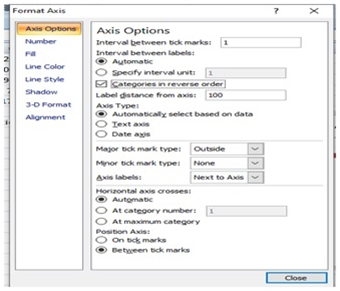
® Step 11÷ click on the list of tasks in the left part of the chart, a format axis window will be opened. Select on categories in reverse order option under axis options then click on ok or close.
Out come
Step
12÷ below start date and right on any of the cell [ table]. A window will
appear, click on format cell go to general and copy the number you see there.
Step 13÷ right click on any of the date above. A
small window will appear click on format axis. Under axis option change major
unit and minor unit to fixed then add the number you want for the date
intervals. The change minimum to fix and then input the number you copied.
® Step
14÷
in order to remove excess space right click on any of the orange bar and select
on format data series. In the format data series set separated to 100% and gap
to 0% the click on close or ok.
This will be the outcome;
Steps 15÷ in order to make you
work more attractive right click on the red bar then click on format data
series. Go 3 D format and reset the width and height of top to be 6pt then
click on close.
This will be the outcome;
 |
| ENDS OF GANTT CHART |
CREATION
OF MULTIPLICATION
TABLE
In order to create a multiplication table you need
to make use of mixed formula. Mixed formula is an example of formulas which is
used in Microsoft excel to solve mathematical problem. It makes use of dollar
sign in the beginning and middle of the calculation e.g. = ($A2-B$2), = ($A1+C$3), = ($C2*B$2).
STEPS
TO CREATE A MULITIPLICATION TABLE
1.
1.
Go to the first cell and input
‘=($A2*B$1)’ click on enter the answer will be displayed.
PREPARATION OF
RESULT SHEET USING MICROSOFT EXCEL
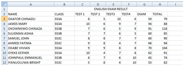
STEP 1: fill in the name of the student, test
scores and examination score
STEP 2: go
to the next row after the examination score row and input total. Use this
formula to get the total ‘=SUM (C2:G2)
STEP 3: Drag the answered box down word
This will be the outcome
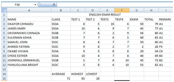
STEP 4: in order to get the average use this
formula =average (H3:H12)
STEP 5: in order to get highest score use this
formula =MAX (H2:H12)
STEP 6: to
get the lowest score use this formula=MIN (H2:H12)
Out come
e.g.
=IF(H3<40,"F9",IF(H3<46,"D7",IF(H3<51,"P",IF(H3<56,"C6",IF(H3<61,"C4",IF(H3<66,"C2",IF(H3<71,"B3",IF(H3<76,"B2",IF(H3>76,"A1")))))))))
=IF(H10<40,"F9",IF(H10<46,"D7",IF(H10<51,"P",IF(H10<56,"C6",IF(H10<61,"C4",IF(H10<66,"C2",IF(H10<71,"B3",IF(H10<76,"B2",IF(H10>76,"A1")))))))))
Your
result sheet is ready


